OCT Today
For now, OCT is most useful when a patient is either a glaucoma suspect or has early-to-moderate disease, as a tool for helping to detect damage and progression (or conversion from glaucoma suspect or ocular hyperten-sive to glaucoma). While there are many parallels between OCT technology and visual fields—for example, being able to use them for either event-based analysis or trend-based progres-sion analysis—OCT is arguably a better tool for use in early disease, because when we test visual function with a visual field test, the plasticity and overlap inherent in the visual system tend to compensate for any early damage. As a result, early dam-age may be picked up by an OCT scan rather than by a visual field test.
On the other hand, late in the dis-ease OCT is less useful because of the “floor effect,” which refers to the fact that when the nerve fiber layer thickness reaches about 45 to 50 µm, it bottoms out and doesn’t decrease any further—even though damage caused by the disease may continue to worsen. Once you reach that level, there’s really no point in using OCT to detect progression; if you do, it may give you a false sense of security that there’s no change happening when the patient may actually be getting worse. At that point we usually rely on visual fields and other functional testing to determine whether progression is occurring.
This limitation of OCT measurements could change in the future, because there’s some evidence that other OCT parameters such as the thickness of the macular ganglion cell complex may still reveal change in more advanced disease. (Some studies are currently exploring that possibility.) In addition, a newer technology called OCT angiography, or OCTA, which uses OCT to map the blood vessels in the retina, might also turn out to be helpful in advanced disease.
OCT gives us a wealth of data to work with, because it can provide structural information about many parts of the retina and optic nerve head—and now the lamina cribrosa—while OCTA can look at the retinal and peripapillary blood vessels. In fact, one of our jobs over the next five years is to figure out which information provided by OCT is important at which stage of the disease. We may end up focusing on one group of OCT parameters in early disease and a different group in more advanced disease.
Factors Affecting OCT Accuracy
A number of things can undermine the accuracy of an OCT scan. To avoid basing a medical decision on poor data, be mindful of these five factors:
• Signal quality. The quality of the data in an OCT scan depends, among other things, on signal strength. Fortunately, OCT systems measure the signal-to-noise ratio of the data being received and give us a number gauging the scan quality after each measurement.
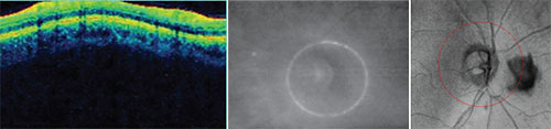 |
| Potential problems that can undercut the accuracy of your scan. Left: The depth of the scan must be correct. Here, the display is cut off at the top because of inaccurate scan depth. The instrument may interpret the missing data as 0-µm thickness at that location. Center: If the optic nerve is not centered in the scan circle, thickness measurements will be thrown off, giving the impression of a focal defect that doesn’t exist. Right: Opacities such as this floater will disrupt the data because the instrument can’t measure through them. |
Signal strength can be decreased for a variety of reasons; the most common reasons are cataract, media opacities, corneal edema, vitreous floaters and dry eye. The latter is easy to treat, so if you get poor signal strength and the media appear clear, give the patient artificial tears right before the next scan. That often improves signal strength significantly. Lower signal strengths will often yield lower retinal nerve fiber layer thickness values that will improve with re-scanning to yield higher (and probably more accurate) values.1
Movement and blinking artifacts can also be a problem because they interrupt the scans. This is becoming less of a problem as OCT instruments scan faster, but it’s still a potential issue. You may observe these movements if you’re watching the patient, but if not, you may note a break or a horizontal line in the gray-scale image of the optic nerve and retina. It may look like the top half and bottom half don’t line up. That means the patient moved or blinked.
Using the Zeiss Cirrus spectral-domain OCT, we consider a scan-quality reading of 7 out of 10 (or better) to mean that the scan contains reliable, useful information. (Other manufacturers also have minimum signal strength guidelines that are considered necessary to perform analysis.) Checking the scan-quality number before you rely too much on the data is important, because the OCT will give you an analysis even if the scan had poor signal strength.
If you do find that the scan was of poor quality, then you need to figure out the reason. In that situation, every box on the OCT readout tells you something—even the parts that people don’t pay much attention to, like the TSNIT graph overlay between the two eyes, and the segmentation section at the bottom.
• Scan alignment. Not only does the eye have to be aligned on the visual axis, but the depth of the scan has to be correct. You can see whether or not it’s correct in the colored graph where the retinal data is presented as a sinusoidal pattern. The graph should be aligned centrally in the box. If it’s too high or too low—too high is most common—then the scan was cut off, and you’ll be missing data for that section, which the instrument will interpret as 0-µm thickness in that area. (See the sample scan shown above, left.) That’s certainly going to disrupt your data and make values less than they should be. This type of scan alignment error is quite common in eyes with high axial myopia.
• Scan centration. When the scan circle isn’t centered around the optic nerve (see example, above, center), the part of the circle that’s too close to the nerve will measure thicker than it actually is, and the part that’s farther away from the center will measure thinner. As a result, you may think there’s a focal defect in the thin area. This problem usually occurs when the patient has difficulty maintaining fixation. The instrument may be centered properly at first, but then the patient moves a little or the eye shifts. A good technician will pick this up and instruct the patient to refixate.
This is an error that you won’t pick up by looking at the scan quality and signal strength. The signal strength may be excellent, but if the scan is not centered properly, you’re going to get misleading measurements. Fortunately, this error is becoming less common with the newer-generation OCT devices that have an auto-tracking feature to maintain scan centration.
• Opacities. These are usually floaters. (See example, above, right) Floaters will disrupt the scan, because OCT technology can’t measure through them. This is a problem that’s often easy to fix, however; you can have the patient look away and look back. That will usually move the floater out of the field of view, or at least outside of the scan circle.
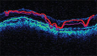 |
| OCT software will try to show the segments of the retinal nerve fiber layer, but low scan quality can produce a garbled result. |
• Segmentation errors. The software will try to segment out the retinal nerve fiber layer, but if the scan quality isn’t good, the segmentation will be thrown off and lead to inaccurate values. (See example, above.)The retinal nerve fiber layer is sup-posed to be the area between the two red lines. Anything that affects scan quality can cause this type of error.
Event-based or Trend-based?
There are two basic strategies for detecting change over a series of tests: event-based analysis and trend-based analysis. Each has advantages and limitations, so it’s important to understand the difference.
• Event-based analysis. To perform event-based analysis, you simply compare one test to another. The practical reality is that there’s a measurement error in every test we do, so in order to decide whether a change has actually occurred between the two tests, you have to first decide what amount of change in the measurements is likely to be greater than the instrument’s potential error. Some current studies indicate that spectral-domain-OCT has about a 4-µm intervisit reproducibility.2 So, to be sure a change is real, it should be greater than twice that, or 8 µm (approximately twice the statistical standard deviation value).
In our practice, we’ve chosen to be conservative and look for change greater than 10 µm; if we don’t see a 10-µm change, we take the result with a grain of salt. However, certain things can lower our threshold for detection. If a patient has a very thin cornea, for example, that tells me that the patient may be at greater risk. In that case I’ll lower my benchmark for progression to 8 µm.
Note that
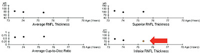 |
| Trend-based analysis looks at a series of sequential test results over time. Here, three of four parameters have remained stable, but one has changed significantly, which the software has highlighted by coloring the circle orange. |
Event-based analysis has some notable limitations: It’s susceptible to outliers, and it may identify false progression. On the other hand, it’s easy. That’s why many doctors use this kind of analysis in practice, especially if they don’t have glaucoma progression analysis software, which features trend-based analysis.
• Trend-based analysis. This approach looks at a series of sequential tests, including your baseline tests, and measures the slope of change over time for whatever parameter you’re looking at—overall change, change in the superior or inferior segments, or change in the ganglion cell complex. It’s primarily concerned with the rate of change rather than the amount. (This is analogous to visual field progression detection.) As you can see in the example on the facing page, three of four parameters have remained relatively stable in this eye, but one has changed significantly over time. The software has highlighted this by turning the circle that represents that measurement orange.
The advantage of trend-based analysis is that it’s less susceptible to fluctuation because it’s looking at change over a period of time. The disadvantage is that it requires a large number of tests. In addition to your baseline tests, you usually need at least two or three subsequent tests to compare to your baseline to make the trend statistically robust. If you only get one scan a year, it can take several years to detect change using this type of analysis. Furthermore, to allow valid comparisons, it’s critically important to choose baseline scans that were performed with good scan parameters.
In general, trend-based analysis is preferable to event-based analysis. However, there are many situations in which trend-based analysis can’t help—even if it’s available in software like Zeiss’s Guided Progression Analysis. For example, a new patient may have had an OCT done on one ma-chine and now you’re doing it on another. Or you may have recently upgraded from one OCT to a newer one, perhaps from time-domain to Fourier-domain. Those two types of OCT data can’t be directly compared. Practical issues like these often force us to resort to event-based analysis.
Helpful Strategies
These strategies will help you get the most from your OCT data:
• Look at the entire readout, not just one or two numbers. Many surgeons pick out one or two key numbers and only look at those when they review a scan. But you have to look at the entire scan to make sure the quality is good and the scan is centered. We try to discipline ourselves to avoid looking at the nerve fiber layer thickness—overall, inferior and superior—until after we review all of the other parameters, to make sure the scan has good-quality data.
This is part of the reason for the problem referred to as “red disease,” where patients get referred—and sometimes treated—for glaucoma because they appear to have an abnormal OCT. When you look at the OCT, you find there’s something wrong with the scan, not the patient. OCT is a powerful tool, but it’s up to the clinician to use it correctly.
• Look for focal change, not just overall change. It’s important to remember that retinal nerve fiber layer thinning can happen in several ways, which will be reflected in different scores. For example, you may find a global, overall decrease in average thickness, or you may find a focal decrease in one quadrant. The three most common RNFL progression patterns are:
— a new RNFL defect;
— widening of an existing defect;
— deepening of an existing RNFL defect without widening.
Studies have looked at these changes, and all of them seem to be important as a means to detect glaucoma.3 In practice, some doctors are in the habit of just looking at the overall thickness number; but for monitoring progression, if there’s already a defect, you want to look at that area for changes. (The pie charts on the readout will tell you if a focal defect is getting worse.) That’s important, because if a focal defect gets worse it may not cause much of a difference in the overall thickness, leading you to miss the change.
 |
| Guided Progression Analysis shows focal areas of change or loss in yellow. |
• Be sure to account for normal aging. There’s a small loss of retinal nerve fiber layer and ganglion cells as we age, even in the healthiest of individuals, so it’s important to take this into account when diagnosing or monitoring progression to avoid mistaking normal aging for disease. To do that, we need to know what the rate of normal loss is—at least on average.
Different studies have looked at this, both in a cross-sectional manner (taking a population and dividing it up into decades or five-year periods and looking at the average NFL thickness of normal patients in each age group) and longitudinal fashion (where individuals are followed over time). One study recruited 100 normal in-dividuals for cross-sectional analysis and 35 for longitudinal analysis.4 That study found a loss of 0.33 µm per year using cross-sectional data and 0.52 µm per year using longitudinal. The Advanced Imaging for Glaucoma Study did both types of analysis with 192 eyes over five years. The cross-sectional analysis found a GCC loss of 0.17 µm per year and overall retinal nerve fiber layer loss of 0.21 µm per year; the longitudinal analysis found a loss of 0.25 µm per year in GCC thickness and 0.14 µm in overall nerve fiber layer thickness.5 (Obviously, longitudinal data is likely to be more robust, but longitudinal studies don’t go on long enough to cover the age span that can be covered in a cross-sectional study.)
Many people combine the cross-sectional data and longitudinal data and average them. Conservatively, you’re looking at about 0.2 µm per year for the NFL thickness. That’s not a lot of loss, but over 10 years that can add up to several microns of change. As a result, that has to be factored into the software designed to analyze these data and taken into account when you’re looking into progression without the help of software. So if you’re not using the GPA software and you’re comparing two scans five years apart, trying to decide whether the patient has progressed or not, you need to be aware of that possible age-related change.
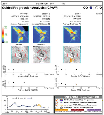
Using GPA
Zeiss’s GPA is one of the programs commonly used to help analyze OCT results. The printout includes thickness charts at the top, in color; the change graphs for different parameters appear below that; and at the bottom left there’s a chart that overlays the TSNIT pattern from multiple tests so you can identify any focal areas of change or loss. (See example, right) When the printout shows a yellow marker, that means it detects significant progression in that parameter; if it’s red, that means the progression has been confirmed by multiple tests. In this example, the printout indicates progression of an inferior defect, noted in three different places on the printout: the area is illuminated in yellow on the black and white change map for exam #3; it’s also represented by a yellow dot in the inferior segment thickness change graph; and it’s colored yellow in the TSNIT graph in the lower left.
The GPA also allows you to do event-based analysis, which is sometimes useful for comparing to trend-based analysis. The readout provides a chart that shows the scores from different tests. However, as with most event-based analyses, you have to be careful. Consider the two examples on the following page (p.58). In the example on the left, the highlighted boxes are parameters that appear to be significantly changed. However, if you compare this to the trend analysis over time (as shown in the images above the boxes), there is no significant change.
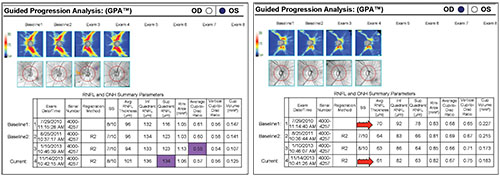 |
| Differences between individual numbers may suggest that significant change has taken place, but a closer examination of the larger picture, including trend analysis, may show that a significant change has not actually occurred. |
The second example shows that the average RNFL thickness in this eye has decreased from 70 µm to 61 µm. You might say that’s significant; it is 9 µm of change. But if you look at reference baseline exams 1 and 2, there’s some variability between them, meaning the value of 70 µm should be taken with a grain of salt, and the amount of change may be less than it appears. Again, these examples demonstrate why trend-based analysis is generally preferable to event-based analysis—as long as you have sufficient data to use trend-based analysis.
Which Parameters Matter Most?
This is a challenging question that’s being looked at by a number of researchers. One reason this is important is that if you have two conflicting parameters—perhaps one looks stable while the other appears to have progressed—having a sense of which parameter is known to be associated more strongly with progression will help you judge which parameter should have more impact on your decision.
Another issue is that doctors would prefer to look at one or two things rather than a field of information when making a clinical decision. Knowing which parameters are most associated with progression should make it possible to create an index that incorporates those particular parameters, allowing doctors to get the most reliable information in a single number. Admittedly, it’s always dangerous to give people a single thing to look at—we might be encouraging them to ignore something else that’s important. But it’s better to have a composite index that takes different things into account than to only look at one piece of data, such as change in average thickness.
Our group conducted a sub-study under the Advanced Imaging for Glaucoma Study in which we identified different parameters that appeared to be especially useful for detecting progression. (We defined progression as visual field progression, to use a marker not related to nerve fiber layer change.) For example, we looked at different retinal nerve fiber layer parameters like focal loss volume; overall inferior quadrant volume; and all of the ganglion cell complex parameters. We found that one of the most sensitive predictors of progression is focal loss volume, both in the GCC and RNFL. (This supports the premise that focal change is able to detect progression earlier than overall average thickness changes.) Using that finding in concert with other relevant data, we created something we call the Glaucoma Composite Progression index. The GCP index combines structural measurements such as central corneal thickness and GCC focal loss volume with patient parameters such as age.
So far, our attempts (and many others’) are still just research; they haven’t been incorporated into any instruments. But based on our own work, we can at least say that doctors should be monitoring the GCC focal loss volume. That parameter was better at predicting change than the other focal loss or overall loss measurements your instrument may provide.
Making the Most of OCT
To summarize, there’s no question that OCT can help us diagnose and monitor our glaucoma patients, especially those with early or moderate disease. But you’ll get the most out of your OCT scans if you:
• maintain good quality readings by monitoring scan signal quality and the alignment and centration of the scan, and watch out for opacities and segmentation errors;
• look at the entire readout, not just one or two numbers;
• look for focal change, not just overall change;
• remember to account for the aging effect; and
• use trend-based analysis whenever possible. And when you need to use event-based analysis, be aware of its potential problems so you get the best possible information from the data comparison. REVIEW
Dr. Francis is a professor of ophthalmology in the glaucoma service and the Rupert and Gertrude Stieger Endowed Chair at the Doheny Eye Institute, Stein Eye Institute, David Geffen School of Medicine, University of California Los Angeles. Dr. Chopra is the medical director of the Doheny Eye Centers Pasadena and an associate professor of ophthalmology of the glaucoma service in the department of ophthalmology at the David Geffen School of Medicine at UCLA. He is also the director of glaucoma research at the Doheny Image Reading Center at the Doheny Eye Institute. Drs. Francis and Chopra have no financial ties to any product mentioned.
1. Wu Z, Vazeen M, Varma R, Chopra V, Walsh AC, LaBree LD, Sadda SR. Factors associated with variability in retinal nerve fiber layer thickness measurements obtained by optical coherence tomography. Ophthalmology 114:1505-1512, 2007.
2. Mwanza JC, Chang RT, Budenz DL, et al. Reproducibility of peripapillary retinal nerve fiber layer thickness and optic nerve head parameters measured with cirrus HD-OCT in glaucomatous eyes. Invest Ophthalmol Vis Sci 2010;51:5724-5730.
3. Leung CK, Yu M, Weinreb RN, Lai G, Xu G, Lam DS. Retinal nerve fiber layer imaging with spectral-domain optical coherence tomography: Patterns of retinal nerve fiber layer progression. Ophthalmology 2012;119:9:1858-66.
4. Leung CK, Yu M, Weinreb RN, Ye C, Liu S, Lai G, Lam DS. Retinal nerve fiber layer imaging with spectral-domain optical coherence tomography: A prospective analysis of age-related loss. Ophthalmology 2012;119:4:731-7.
5. Zhang X, Francis BA, Dastiridou A, Chopra V, Tan O, Varma R, Greenfield DS, Schuman JS, Huang D; Advanced Imaging for Glaucoma Study Group. Longitudinal and cross-sectional analyses of age effects on retinal nerve fiber layer and ganglion cell complex thickness by fourier-domain OCT. Transl Vis Sci Technol 2016;4:5:2:1.